Written by Atrebas
on March 7, 2021

Comparison of different for loops methods in parallel distance computation with R, C, and OpenMP

The title is a bit long, but I’ll try to keep the post short. In my previous post, I presented how to convert a linear index to lower triangular subscripts. As an example, it can be useful for distance computation. Rather than using two loops for each row being compared in the input matrix, it is possible to use a single loop on an index, and then compute the indices of the evaluated rows.
In a standard parallel distance implementation using two loops, all the computations are done for the first row, then the second, … I once heard that it could lead to a concurrency issue and limit the performance.
Using an index, we can proceed with a ‘diagonal-wise’ numbering, the combinations being computed in parallel are then more likely to involved different rows, and this may consequently limit a putative concurrency phenomenon. That’s what I aimed to check in this article.

The pmdr package

I wrote a toy R package, named pmdr for Parallel Manhattan Distances in R. I focused on manhattan distances because it was easier to implement for this exploratory approach. For simplicity, it only works with integers and missing values are not allowed. Also, the results are returned as a vector.
This package contains three C functions, and the R wrapper. It can be installed from Github as shown below.

# install.packages("remotes")
remotes::install_github("Atrebas/pmdr")

Looping strategies

Using two loops

In the first C function, the loop is performed in a ‘classic’ way, with a loop on i1 and i2, the rows being evaluated. From i1 and i2, k, the index of the combination being evaluated is computed.
I is the number of rows of the input matrix ptx and ptres is the output vector.
Note that the loop on j corresponds to the columns of the input matrix.

for (i1 = 1; i1 < I; i1++) {                               // loop on row 1
  for (i2 = 0; i2 < i1; i2++) {                            // loop on row 2
    k = K - (I - i2) * ((I - i2) - 1) / 2 + i1 - i2 - 1;   // compute the index
    ptres[k] = 0;
    for (j = 0; j < J; j++) {                              // loop on the columns 
      ptres[k] += abs(ptx[i1 + I * j] - ptx[i2 + I * j]);  // increment the Manhattan distance
    }
  }
}

Using one loop, colwise

In the second C function, a loop is performed on k, the index of the combination being evaluated. Within this loop, i1 and i2 are determined in a colwise way.

for (k = 0; k < K; k++) {                                 // loop on the index (column-wise)
  ptres[k] = 0;
  kp = K - k - 1;
  p  = floor((sqrt(1 + 8 * kp) - 1) / 2);
  i1 = I - (kp - p * (p + 1) / 2) - 1;                    // compute row 1
  i2 = I - 2 - p;                                         // compute row 2
  for (j = 0; j < J; j++) {                               // loop on the columns
    ptres[k] += abs(ptx[i1 + I * j] - ptx[i2 + I * j]);   // increment the Manhattan distance
  }
}

Using one loop, diagwise

In the third function, the parallelization is done on the linear index k, but this time, the combination of rows used for the computation is determined using diagwise traversal (and the order of the results in the output vector will thus be different from the previous ones).

for (k = 0; k < K; k++) {                                   // loop on the index (diagonal-wise)
  ptres[k] = 0;
  kp = K - k - 1;
  p  = floor((sqrt(1 + 8 * kp) - 1) / 2);
  i1 = I - (kp - p * (p + 1) / 2) - 1;                      // compute row 1
  i2 = i1 - (I - 1 - p);                                    // compute row 2
    for (j = 0; j < J; j++) {                               // loop on the columns
      ptres[k] += abs(ptx[i1 + I * j] - ptx[i2 + I * j]);   // increment the Manhattan distance
    }
}

Example

First, here is how the R function works. As mentioned earlier, I was interested in returning the results as a vector, not a distance matrix.

# remotes::install_github("atrebas/pmdr")

library(pmdr)

n_row <- 7
n_col <- 10

mat   <- matrix(sample(1:30, n_row * n_col, replace = TRUE),
                nrow = n_row,
                ncol = n_col)

mat

##      [,1] [,2] [,3] [,4] [,5] [,6] [,7] [,8] [,9] [,10]
## [1,]    6   17   26   23   15   20   13   11    1    13
## [2,]   25   28    1   12   18    1   10    9   10    12
## [3,]   13   19   16   14    4   16    7   24    8    30
## [4,]   24   22   16   12   20   16    3    1   24    10
## [5,]    8   11   11   21   23    4   21   21    7    25
## [6,]   25   10    5   24    2   16   11   16   16    12
## [7,]   10    3    2   30   22    7   23    8   18    24

distance(mat, loop = "standard")

##  [1] 103  86  99  85  88 110 105  70 100  79 103  95  79  82 124 126  87 123  97
## [20]  59  94

distance(mat, loop = "colwise")

##  [1] 103  86  99  85  88 110 105  70 100  79 103  95  79  82 124 126  87 123  97
## [20]  59  94

distance(mat, loop = "diagwise")

##  [1] 103 105  95 126  97  94  86  70  79  87  59  99 100  82 123  85  79 124  88
## [20] 103 110

Benchmark 1

Running a quick benchmark on my four-core laptop shows no benefit of the colwise and diagwise methods over the basic double loop.

library(pmdr)
library(microbenchmark)

n_row <- 500
n_col <- 1000

mat   <- matrix(sample(1:30, n_row * n_col, replace = TRUE),
                nrow = n_row,
                ncol = n_col)

pmdr::num_procs()

## [1] 4

microbenchmark(standard = distance(mat, loop = "standard"),
               colwise  = distance(mat, loop = "colwise"),
               diagwise = distance(mat, loop = "diagwise"),
               times    = 20L)

## Unit: milliseconds
##      expr      min       lq     mean   median       uq      max neval
##  standard 214.3665 217.3569 219.9808 219.4761 223.6465 226.3603    20
##   colwise 245.2472 245.9105 247.5465 246.4485 246.8566 266.0562    20
##  diagwise 244.0165 250.4270 252.1025 251.4929 252.5880 275.2310    20

Benchmark 2

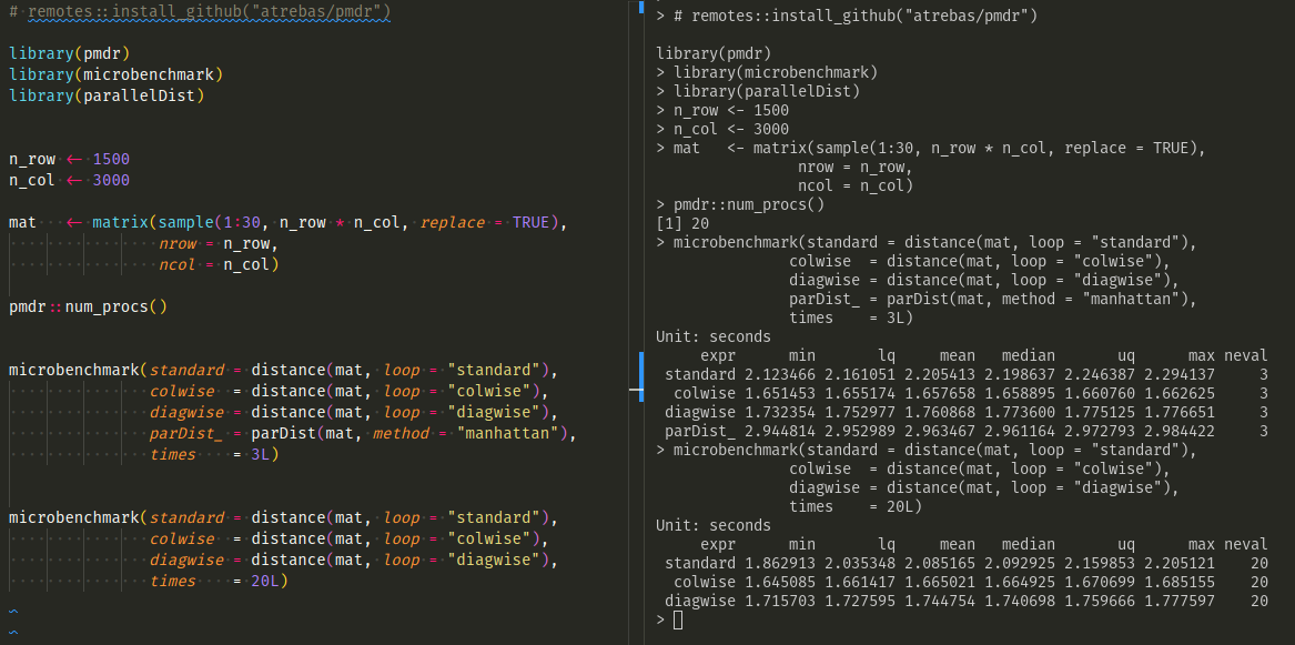
Here is a screenshot of a second benchmark with larger data on a bigger machine (20 cores). In this case, the colwise method seems to perform slightly better, but the benefit would probably vanish if a matrix was returned (because in that case, computing the index in the double loop would be useless).
Also, a quick test with the parallelDist package shows that the timing obtained with pmdr is competitive.

Conclusion

No significant difference was observed between the different methods, but writing the pmdr package was a good refresher on R/C binding and my implementation of distance computation in OpenMP seems to work correctly.

The parallelDist package is much more robust and feature-rich than pmdr, so the comparison is not relevant. Nevertheless, the timing obtained in the benchmark above looks satisfying.

Note: I do not have a CS background. This post is based on MOOCs, reading, inspiration from other people’s work (Drew Schmidt’s Romp package in particular), and a lot of segfault debugging.

← Top