Written by Atrebas
on June 17, 2020

A gentle introduction to data.table

The basics
by
Chaining commands
Recap
More details about DT[, j]
.SD
- Iterate over several columns
- Selecting columns with .SDcols
To infinity and beyond!

data.table is one of the greatest R package. It provides an enhanced version of base R’s data.frame with syntax and feature enhancements, making data manipulation concise, consistent, efficient, and fun!

This post gives a quick introduction to data.table. The main objective is to present the data.table syntax, showing how to perform basic, but essential, data wrangling tasks.

Let’s start by creating a simple data.table.

library(data.table) # version 1.13.0

DT <- data.table(Fruit = rep(c("banana", "apple", "orange"), 3:1),
                 Year  = c(2008, 2009, 2010, 2009, 2010, 2010),
                 Count = 1:6)
DT

##     Fruit Year Count
## 1: banana 2008     1
## 2: banana 2009     2
## 3: banana 2010     3
## 4:  apple 2009     4
## 5:  apple 2010     5
## 6: orange 2010     6

class(DT)

## [1] "data.table" "data.frame"

How we can select the first two rows and the first two columns of a data.table? Well, that’s simple:

DT[1:2, 1:2]

##     Fruit Year
## 1: banana 2008
## 2: banana 2009

In base R, we can access elements of a matrix or a data.frame using the square brackets indexing method. It’s the same with data.table.

To start, think DT[rows, columns], also presented in a short way: DT[i, j]. With data.table, most of the things take place within these square brackets.
The magic is that you can do much more with the simple command DT[i, j]. In particular, rows and columns can be referred to without using any quotes or $ symbol, making the code very clear.

The basics

Operations on rows

For example, to select rows using a condition:

DT[Fruit == "banana", ]                  # select rows where Fruit equals banana

##     Fruit Year Count
## 1: banana 2008     1
## 2: banana 2009     2
## 3: banana 2010     3

DT[Fruit == "banana" & Year > 2008]      # select rows where Fruit equals banana and Year is higher than 2008

##     Fruit Year Count
## 1: banana 2009     2
## 2: banana 2010     3

When performing operations on rows only, the j element is left empty (DT[i,]), as in the first command, or simply ignored (DT[i]) as in the second command.

Likewise, we can order the data:

DT[order(Fruit), ]          # order according to the Fruit column, in ascending order

##     Fruit Year Count
## 1:  apple 2009     4
## 2:  apple 2010     5
## 3: banana 2008     1
## 4: banana 2009     2
## 5: banana 2010     3
## 6: orange 2010     6

DT[order(Fruit, -Year)]     # order according to the Fruit and Year columns, in ascending and descending order, respectively

##     Fruit Year Count
## 1:  apple 2010     5
## 2:  apple 2009     4
## 3: banana 2010     3
## 4: banana 2009     2
## 5: banana 2008     1
## 6: orange 2010     6

Or sample rows:

DT[sample(nrow(DT), 3)]     # randomly sample three rows

##     Fruit Year Count
## 1: banana 2010     3
## 2: banana 2009     2
## 3:  apple 2010     5

The command above can be abbreviated as follows:

DT[sample(.N, 3), ]        # randomly sample three rows

##     Fruit Year Count
## 1: orange 2010     6
## 2:  apple 2010     5
## 3:  apple 2009     4

.N is an alias for the number of rows. data.table offers several syntactic sugars like this, as we will see below.

Operations on columns

Select columns

To select a column, we just specify the name in DT[, j].

DT[, Count]            # select the Count column, returns a vector

## [1] 1 2 3 4 5 6

The previous command returns a vector, if you want the result to be a data.table, you have to use list(), or more simply the . alias.

DT[, list(Count)]       # select the Count column, returns a data.table

##    Count
## 1:     1
## 2:     2
## 3:     3
## 4:     4
## 5:     5
## 6:     6

DT[, .(Count)]          # ditto

##    Count
## 1:     1
## 2:     2
## 3:     3
## 4:     4
## 5:     5
## 6:     6

DT[, .(Fruit, Count)]   # select the Fruit and Count columns

##     Fruit Count
## 1: banana     1
## 2: banana     2
## 3: banana     3
## 4:  apple     4
## 5:  apple     5
## 6: orange     6

To select columns using a vector of column names, one should use the .. prefix. It indicates to search the corresponding vector ‘one level up’ (i.e. in the global environment).

cols <- c("Fruit", "Year")
DT[, ..cols]   # select the columns provided in the cols vector

##     Fruit Year
## 1: banana 2008
## 2: banana 2009
## 3: banana 2010
## 4:  apple 2009
## 5:  apple 2010
## 6: orange 2010

Computation on columns

To apply a function on a column:

DT[, max(Year)]                # sum the Count values

## [1] 2010

DT[, cumsum(Count)]

## [1]  1  3  6 10 15 21

By default, the result is returned as a vector. Just like above with column selection, to obtain the result as a data.table, it is necessary to use .(). Doing so, we can also assign colnames to the result. When no column names are provided, they are automatically generated as V1, V2, …

DT[, .(cumsum(Count))]                # sum the Count values

##    V1
## 1:  1
## 2:  3
## 3:  6
## 4: 10
## 5: 15
## 6: 21

DT[, .(CumsumCount = cumsum(Count))]     # sum the Count values with column name CumsumCount

##    CumsumCount
## 1:           1
## 2:           3
## 3:           6
## 4:          10
## 5:          15
## 6:          21

To apply a function on several columns:

DT[, .(sum(Count), max(Year))]   # sum the Count values and get the maximum Year value

##    V1   V2
## 1: 21 2010

Assigning colunm names and indenting the code:

DT[, .(SUM = sum(Count),
       MAX = max(Year))]         # sum the Count values and get the maximum Year value, assigning column names

##    SUM  MAX
## 1:  21 2010

Modify / Add / Delete columns

Note that the previous commands create a new data.table. To modify an existing column, or create a new one, use the := operator.

DT[, Year := Year + 1]               # modify the Year column
DT[, Cumsum_Count := cumsum(Count)]  # create a new Cumsum_Count column

As you can see below, DT has been modified even if we did not assign the result:

DT

##     Fruit Year Count Cumsum_Count
## 1: banana 2009     1            1
## 2: banana 2010     2            3
## 3: banana 2011     3            6
## 4:  apple 2010     4           10
## 5:  apple 2011     5           15
## 6: orange 2011     6           21

Using the data.table := operator modifies the existing object ‘in place’, which has the benefit of being memory-efficient. Memory management is an important aspect of data.table. There is a dedicated vignette to learn more about it.

The principle is the same to modify or add several columns:

DT[, c("CountX3", "CountX4") := .(Count * 3, Count * 4)]
DT

##     Fruit Year Count Cumsum_Count CountX3 CountX4
## 1: banana 2009     1            1       3       4
## 2: banana 2010     2            3       6       8
## 3: banana 2011     3            6       9      12
## 4:  apple 2010     4           10      12      16
## 5:  apple 2011     5           15      15      20
## 6: orange 2011     6           21      18      24

It is also possible to use the functional form, which, combined with indentation, offers a more readable alternative:

DT[, ':='(CountX3 = Count * 3,
          CountX4 = Count * 4)]
DT

##     Fruit Year Count Cumsum_Count CountX3 CountX4
## 1: banana 2009     1            1       3       4
## 2: banana 2010     2            3       6       8
## 3: banana 2011     3            6       9      12
## 4:  apple 2010     4           10      12      16
## 5:  apple 2011     5           15      15      20
## 6: orange 2011     6           21      18      24

With a predefined vector of column names, the corresponding object must be put in parentheses.

cols <- c("CountX3", "CountX4")
DT[, (cols) := .(Count * 3, Count * 4)]

And finally, to remove columns, we assign them a NULL value:

DT[, Cumsum_Count := NULL]
DT[, c("CountX3", "CountX4") := NULL]

DT

##     Fruit Year Count
## 1: banana 2009     1
## 2: banana 2010     2
## 3: banana 2011     3
## 4:  apple 2010     4
## 5:  apple 2011     5
## 6: orange 2011     6

Operations on both rows and columns

Obviously, the operations on rows and columns can be combined in DT[i, j]. Operations on j are then performed after the condition in i has been applied.

DT[Fruit != "apple", sum(Count)]

## [1] 12

DT[Fruit == "banana" & Year < 2011, .(sum(Count))]

##    V1
## 1:  3

Combining i and j in a same expression is particularly useful because it allows to modify some values only for rows matching the condition in i, or to create a new column, assigning a given value for matching rows, other rows being left as NA.

DT[Fruit == "banana" & Year < 2010, Count := Count + 1] # modify only the matching rows
DT[Fruit == "orange", Orange := "orange"] # add a new column, non-matching rows will be NA

DT

##     Fruit Year Count Orange
## 1: banana 2009     2   <NA>
## 2: banana 2010     2   <NA>
## 3: banana 2011     3   <NA>
## 4:  apple 2010     4   <NA>
## 5:  apple 2011     5   <NA>
## 6: orange 2011     6 orange

by

Now that you are familiar with DT[i, j], let’s introduce DT[i, j, by].
by can somewhat be viewed as a “third virtual dimension”. The data can be aggregated by group using a single additional argument: by. That’s it. How could it be more simple?

Aggregation by group

DT[, sum(Count), by = Fruit]

##     Fruit V1
## 1: banana  7
## 2:  apple  9
## 3: orange  6

A condition or a function call can also be used in by.

DT[, sum(Count), by = (IsApple = Fruit == "apple")]

##    IsApple V1
## 1:   FALSE 13
## 2:    TRUE  9

DT[, .(MeanCount = mean(Count)), by = (OddYear = Year %% 2 == 1)]

##    OddYear MeanCount
## 1:    TRUE         4
## 2:   FALSE         3

Aggregating on several columns is just as simple, with a character vector in by:

DT[, sum(Count), by = c("Fruit", "Year")]

##     Fruit Year V1
## 1: banana 2009  2
## 2: banana 2010  2
## 3: banana 2011  3
## 4:  apple 2010  4
## 5:  apple 2011  5
## 6: orange 2011  6

Or using .(...) in by:

DT[, .(SumCount = sum(Count)), by = .(Fruit, Before2011 = Year < 2011)]

##     Fruit Before2011 SumCount
## 1: banana       TRUE        4
## 2: banana      FALSE        3
## 3:  apple       TRUE        4
## 4:  apple      FALSE        5
## 5: orange      FALSE        6

And here is a full DT[i, j, by] command:

DT[Fruit != "orange", max(Count), by = Fruit]

##     Fruit V1
## 1: banana  3
## 2:  apple  5

Once again, this is just one single argument: by = .... Much more simple and practical than base::tapply() in my opinion. This is one of the key features that got me hooked on data.table.

Code indentation and reordering

Because data.table offers a consise syntax, commands easily fit on a single line. But it is possible to indent the code for more readability and also to reorder the elements (DT[i, by, j]).

DT[Fruit != "orange",   # select the rows that are not oranges
   max(Count),          # then return the maximum value of Count
   by = Fruit]          # for each fruit

##     Fruit V1
## 1: banana  3
## 2:  apple  5

DT[Fruit != "orange",   # select the rows that are not oranges
   by = Fruit,          # then, for each fruit,
   max(Count)]          # return the maximum value of Count

##     Fruit V1
## 1: banana  3
## 2:  apple  5

Modify a data.table by group

In the previous commands, by has been used to aggregate data, returning a new data.table as output. It is of course possible to use by when modifying an existing data.table and to return the output for each observation of the groups.
For example, to add a column with the number of observations for each group (the .N alias mentioned earlier can also be used in j!):

DT[, N := .N, by = Fruit]

Here is another example:

DT[, MeanCountByFruit := round(mean(Count), 2), by = Fruit]

DT

##     Fruit Year Count Orange N MeanCountByFruit
## 1: banana 2009     2   <NA> 3             2.33
## 2: banana 2010     2   <NA> 3             2.33
## 3: banana 2011     3   <NA> 3             2.33
## 4:  apple 2010     4   <NA> 2             4.50
## 5:  apple 2011     5   <NA> 2             4.50
## 6: orange 2011     6 orange 1             6.00

Chaining commands

Commands can be chained together using DT[ ... ][ ... ] “horizontally”:

DT[, MeanCountByFruit := round(mean(Count), 2), by = Fruit][MeanCountByFruit > 2]

##     Fruit Year Count Orange N MeanCountByFruit
## 1: banana 2009     2   <NA> 3             2.33
## 2: banana 2010     2   <NA> 3             2.33
## 3: banana 2011     3   <NA> 3             2.33
## 4:  apple 2010     4   <NA> 2             4.50
## 5:  apple 2011     5   <NA> 2             4.50
## 6: orange 2011     6 orange 1             6.00

Or “vertically”:

DT[, by = Fruit,
     MeanCountByFruit := round(mean(Count), 2)
  ][
     MeanCountByFruit > 2
   ]

##     Fruit Year Count Orange N MeanCountByFruit
## 1: banana 2009     2   <NA> 3             2.33
## 2: banana 2010     2   <NA> 3             2.33
## 3: banana 2011     3   <NA> 3             2.33
## 4:  apple 2010     4   <NA> 2             4.50
## 5:  apple 2011     5   <NA> 2             4.50
## 6: orange 2011     6 orange 1             6.00

Adding an empty [] at the end of a command will print the result. This is useful for example when modifying columns by reference using :=.

DT[, c("Orange", "N", "MeanCountByFruit") := NULL][]

##     Fruit Year Count
## 1: banana 2009     2
## 2: banana 2010     2
## 3: banana 2011     3
## 4:  apple 2010     4
## 5:  apple 2011     5
## 6: orange 2011     6

Recap

Let’s recap the main commands we have seen so far:

# operations on rows
DT[Fruit == "banana", ]
DT[Fruit == "banana" & Year > 2008]
DT[order(Fruit), ]
DT[order(Fruit, -Year)]
DT[sample(.N, 3), ]

# operations on columns
DT[, Count]
DT[, list(Count)]
DT[, .(Count)]
DT[, .(Fruit, Count)]
cols <- c("Fruit", "Year")
DT[, ..cols]
DT[, cumsum(Count)]
DT[, .(cumsum(Count))]
DT[, .(CumsumCount = cumsum(Count))]
DT[, .(sum(Count), max(Year))]
DT[, .(SUM = sum(Count),
       MAX = max(Year))]

# operations on columns (modifying the data.table)
DT[, Cumsum_Count := cumsum(Count)]
DT[, ':='(CountX3 = Count * 3,
          CountX4 = Count * 4)]
cols <- c("CountX3", "CountX4")
DT[, (cols) := .(Count * 3, Count * 4)]
DT[, Cumsum_Count := NULL]

# operations on both rows and columns
DT[Fruit != "apple", sum(Count)]
DT[Fruit == "banana" & Year < 2011, .(sum(Count))]
DT[Fruit == "banana" & Year < 2010, Count := Count + 1]
DT[Fruit == "orange", Orange := "orange"]

# aggregation by group
DT[, sum(Count), by = Fruit]
DT[, sum(Count), by = (IsApple = Fruit == "apple")] 
DT[, sum(Count), by = c("Fruit", "Year")]
DT[, .(SumCount = sum(Count)), by = .(Fruit, Before2011 = Year < 2011)]
DT[Fruit != "orange",
   max(Count),
   by = Fruit]
DT[, N := .N, by = Fruit]
DT[, MeanCountByFruit := round(mean(Count), 2), by = Fruit]

# chaining
DT[, MeanCountByFruit := round(mean(Count), 2), by = Fruit][MeanCountByFruit > 2]
DT[, c("Orange", "N", "MeanCountByFruit") := NULL][]

That’s the beauty of data.table: simplicity and consistency. DT[rows, columns, by].
No quoted column names, no $ symbol, and no new function. The only new thing is :=, used to assign column(s) by reference. .() is just an alias for list() and .N is an alias for the number of rows.

When we look at the commands above, it appears that data.table is so expressive that very little code is needed. In fact, with so much little text and a regular alignment, brackets, commas, and symbols somehow stand out. Removing the “uncessary” stuff makes the structure more visible. This structure is a guide to read data.table code. I think data.table is more about understanding than memorizing.

# DT[operation on rows, ]
# DT[, operation on columns]
# DT[, .(extract or compute new columns)]
# DT[, newcolumn := assignment]
# DT[, some computation, by = group]
# ...

More details about `DT[, j]`

So far DT[, j] has been used to select, modify, summarize, or compute new columns. But it is even more flexible: the j element can be any arbitrary expression, or set of expressions written within curly braces. For example:

DT[, 1 + 1]

## [1] 2

DT[, plot(Year, Count)]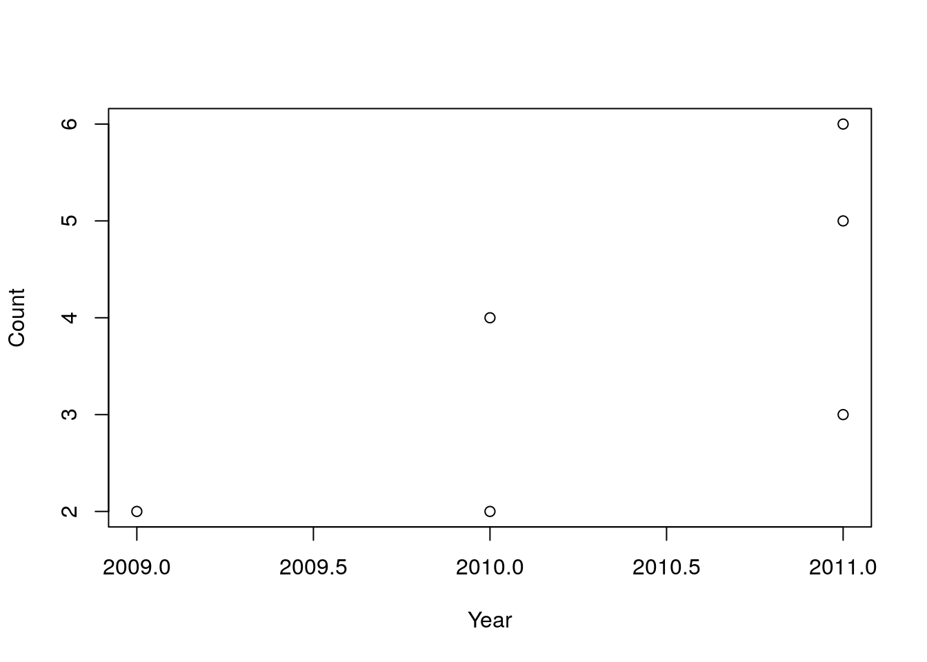

## NULL

DT[, {sum_count <- sum(Count)
      print("The sum of the Count column is:")
      sum_count}]

## [1] "The sum of the Count column is:"

## [1] 22

Note that passing several expressions within curly braces is valid base R code to evaluate several commands, but only return the last result:

{sum123 <- sum(1:3); 1 + 2; sum123}

## [1] 6

Also, as long as the j expression returns a list of equal-length elements (or elements of length one), each element of the list will be converted to a column in the resulting data.table. This is important! Keep that in mind, we’ll see the implication in the next section. But note that it also explains why we used the list() alias .() earlier for operations on columns.

DT[, list(1:3, 4:6, 7)]

##    V1 V2 V3
## 1:  1  4  7
## 2:  2  5  7
## 3:  3  6  7

DT[, {2 + 3             # this command is evaluated but not returned
      list(Col1 = 1:3,
           Col2 = 4:6,
           Col3 = 7)}]

##    Col1 Col2 Col3
## 1:    1    4    7
## 2:    2    5    7
## 3:    3    6    7

.SD

Just like .N is an alias refering to the number of rows, .SD is an alias refering to the Subset of Data for each group, excluding the column(s) used in by. Said differently, .SD corresponds to “the current data for the current group (excluding grouping variables)”. It offers a convenient way to iterate over the columns of a data.table.

To better see it, just print it!

DT[, print(.SD), by = Fruit]

##    Year Count
## 1: 2009     2
## 2: 2010     2
## 3: 2011     3
##    Year Count
## 1: 2010     4
## 2: 2011     5
##    Year Count
## 1: 2011     6

## Empty data.table (0 rows and 1 cols): Fruit

If there is no by, then .SD is DT itself.

DT[, .SD]

##     Fruit Year Count
## 1: banana 2009     2
## 2: banana 2010     2
## 3: banana 2011     3
## 4:  apple 2010     4
## 5:  apple 2011     5
## 6: orange 2011     6

Iterate over several columns

To run a function over all the columns of a data.table, we can use the following expression:

DT[, lapply(.SD, min)]

##    Fruit Year Count
## 1: apple 2009     2

Let’s take some time to explain it step by step:
- iterating over the columns of a data.frame using lapply() is a valid base R expression (e.g. lapply(mtcars, min))
- DT[,j] can take any arbitrary expression as mentioned earlier, so lapply(.SD, min) is used as the j expression
- .SD is, once again, just an alias for the subset of data for each group - no group is used in this first example, so .SD contains all the DT columns)
- iterating over the columns of .SD using lapply obviously returns a list
- as described in the previous section, as long as the j expression returns a list (of equal-length or length-one elements), each element of the list will be converted to a column in the resulting data.table
- so finally, the command above returns a data.table with the minimum value for each column of .SD

Let’s run the same expression, this time by group:

DT[, lapply(.SD, min), by = Fruit]

##     Fruit Year Count
## 1: banana 2009     2
## 2:  apple 2010     4
## 3: orange 2011     6

And of course, we can also select the rows using a DT[i, j, by] command:

DT[Fruit != "apple", lapply(.SD, min), by = Fruit]

##     Fruit Year Count
## 1: banana 2009     2
## 2: orange 2011     6

It is possible to append the result of the aggregation to the current data.table, the values will then be recycled for each observation of a given group:

DT[, c("MeanYear", "MeanCount") := lapply(.SD, mean),
     by = Fruit]
DT

##     Fruit Year Count MeanYear MeanCount
## 1: banana 2009     2   2010.0  2.333333
## 2: banana 2010     2   2010.0  2.333333
## 3: banana 2011     3   2010.0  2.333333
## 4:  apple 2010     4   2010.5  4.500000
## 5:  apple 2011     5   2010.5  4.500000
## 6: orange 2011     6   2011.0  6.000000

Selecting columns with `.SDcols`

By default, .SD contains all the columns that are not provided in by. To run a function on specific columns, use .SDcols to pass a vector of colnames.

DT[, lapply(.SD, min), by = Fruit, .SDcols = c("Count", "MeanCount")]

##     Fruit Count MeanCount
## 1: banana     2  2.333333
## 2:  apple     4  4.500000
## 3: orange     6  6.000000

selected_cols <- "Year"
# indenting the code
DT[, by = Fruit,               # for each fruit
     lapply(.SD, min),         # retrieve the min value
     .SDcols = selected_cols]  # for each column provided in the selected_cols vector

##     Fruit Year
## 1: banana 2009
## 2:  apple 2010
## 3: orange 2011

A regular expression can also be passed using patterns():

DT[, lapply(.SD, min),
     by = Fruit,
     .SDcols = patterns("^Co")]

##     Fruit Count
## 1: banana     2
## 2:  apple     4
## 3: orange     6

Alternatively, a function can be provided in .SDcols. This function must return a boolean signalling inclusion/exclusion of the column:

DT[, lapply(.SD, min),
     by = Fruit,
     .SDcols = is.integer] # !is.integer can also be used

##     Fruit Count
## 1: banana     2
## 2:  apple     4
## 3: orange     6

foo <- function(x) {is.numeric(x) && mean(x) > 2000}
DT[, lapply(.SD, min),
     by = Fruit,
     .SDcols = foo]

##     Fruit Year MeanYear
## 1: banana 2009   2010.0
## 2:  apple 2010   2010.5
## 3: orange 2011   2011.0

To infinity and beyond!

In this post, we have introduced the data.table syntax to perform common data wrangling operations. Nevertheless, we’ve only scratched the surface. data.table offers tens of other impressive features. Here are some more reasons why it deserves to be in your data science toolbox.

data.table has been created in 2006 and is still actively maintained on github, with a responsive, welcoming, and insightful support.
data.table is reliable. A lot of care is given to maintain compatibility in the long run. R dependency is as old as possible and there are no dependencies on other packages, for simpler production and maintenance.
data.table is very reliable. It is a masterpiece of continuous integration and contains more than 9000 tests that you can run locally using test.data.table() to make sure everything works fine with your own settings. There is more test code in data.table than there is code.
while data.table performance is impressive, it is not only for ‘large data’. Why analyzing ‘small data’ should be less convenient than analyzing ‘large data’? data.table is great, even for a six-row dataset like the one used in this post.
data.table offers the fread and fwrite functions, the fastest, most robust and full-featured functions to read or write text files.
data.table offers keys and indices, which are mechanisms that make row subsetting (and joins) blazingly fast.
data.table can perfom the most common data joins as well as advanced joins like non-equi joins or overlap joins.
data.table also include dcast(), melt(), as well as a bunch of utility functions, for efficient and versatile data reshaping.
all these data manipulations are fast (see benchmark), memory-efficient, and just as easy to perform as the few commands presented in this document.
and last but not least, data.table has a nice and fun logo! R! R! R!

Happy data.tabling!

sessionInfo()

## R version 3.6.3 (2020-02-29)
## Platform: x86_64-pc-linux-gnu (64-bit)
## Running under: Ubuntu 18.04.4 LTS
## 
## Matrix products: default
## BLAS:   /usr/lib/x86_64-linux-gnu/blas/libblas.so.3.7.1
## LAPACK: /usr/lib/x86_64-linux-gnu/lapack/liblapack.so.3.7.1
## 
## locale:
##  [1] LC_CTYPE=en_US.UTF-8       LC_NUMERIC=C              
##  [3] LC_TIME=fr_FR.UTF-8        LC_COLLATE=en_US.UTF-8    
##  [5] LC_MONETARY=fr_FR.UTF-8    LC_MESSAGES=en_US.UTF-8   
##  [7] LC_PAPER=fr_FR.UTF-8       LC_NAME=C                 
##  [9] LC_ADDRESS=C               LC_TELEPHONE=C            
## [11] LC_MEASUREMENT=fr_FR.UTF-8 LC_IDENTIFICATION=C       
## 
## attached base packages:
## [1] stats     graphics  grDevices utils     datasets  methods   base     
## 
## other attached packages:
## [1] data.table_1.13.0
## 
## loaded via a namespace (and not attached):
##  [1] compiler_3.6.3  magrittr_1.5    bookdown_0.16   tools_3.6.3    
##  [5] htmltools_0.4.0 yaml_2.2.0      Rcpp_1.0.3      stringi_1.4.3  
##  [9] rmarkdown_2.0   blogdown_0.17   knitr_1.26      stringr_1.4.0  
## [13] digest_0.6.23   xfun_0.11       rlang_0.4.6     evaluate_0.14

← → Top