on
Learning Japanese with data.table and ggplot2
This post is about drawing hiragana and katakana tables using R, data.table, and ggplot2. The objective was to better illustrate the rules that underlie these two Japanese writing systems.
Overview of the Japanese writing systems
For a more detailed and accurate information, Wikipedia articles are excellent and have been used as a source for this article.
There are three Japanese writing systems: the kanji and two kana systems: hiragana and katakana. Rōmaji, the Latin alphabet used to write the Japanese language, is sometimes considered as a fourth system.
Kanji
Kanji (漢字) correspond to Chinese characters adapted for Japanese.
Kanji are logograms: characters represent a word, but can have multiple meanings and most of the time have multiple pronunciations.
There are several tens of thousands of kanji, but approximately 2000 are commonly used to write nouns, as well as stems of verbs, adjectives, and adverbs. They are also used to write Japanese personal names.
Here are a few examples:
- 木, tree, pronounced ki
- 針, needle + 鼠, rat/mouse = 針鼠, hedgehog (a mouse with needles!), pronounced harinezumi
- 田, ricefield + 中, middle = 田中, Tanaka, the fourth most common Japanese surname
Kana
Both for simplification and to better capture the Japanese language specificities, two writing systems have been derived from the kanji: the kana, with hiragana and katakana.
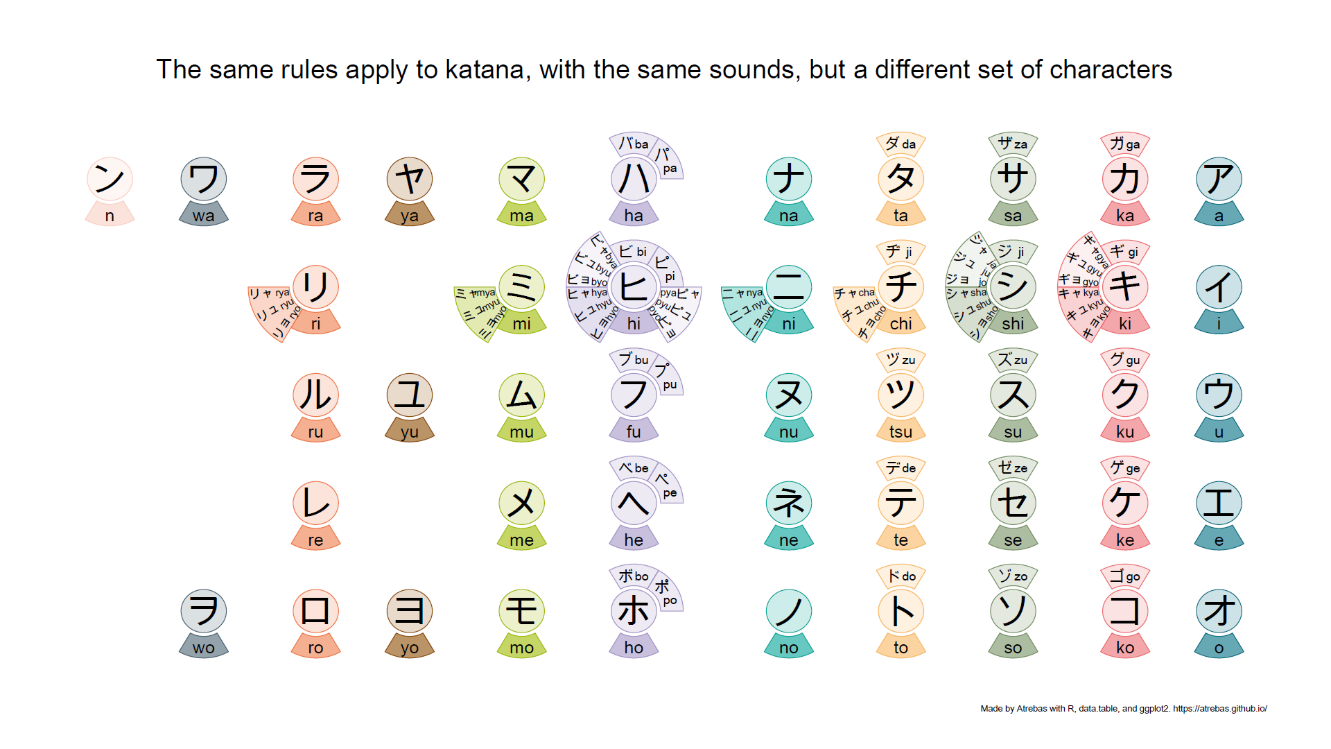
Kana are syllabic systems, each character corresponds to one sound. Hiragana and katakana represent the same sounds but with differents sets of characters. Like kanji, each kana has a given number of strokes and must be written in a precise order.
- Hiragana are used for grammatical elements and Japanese words that have no (simple) kanji. They are also used to indicate kanji pronunciation.
- Katakana are used for transcription of foreign words and the writing of loan words. They are also used for emphasis, in onomatopoeia, or for technical and scientific terms, …
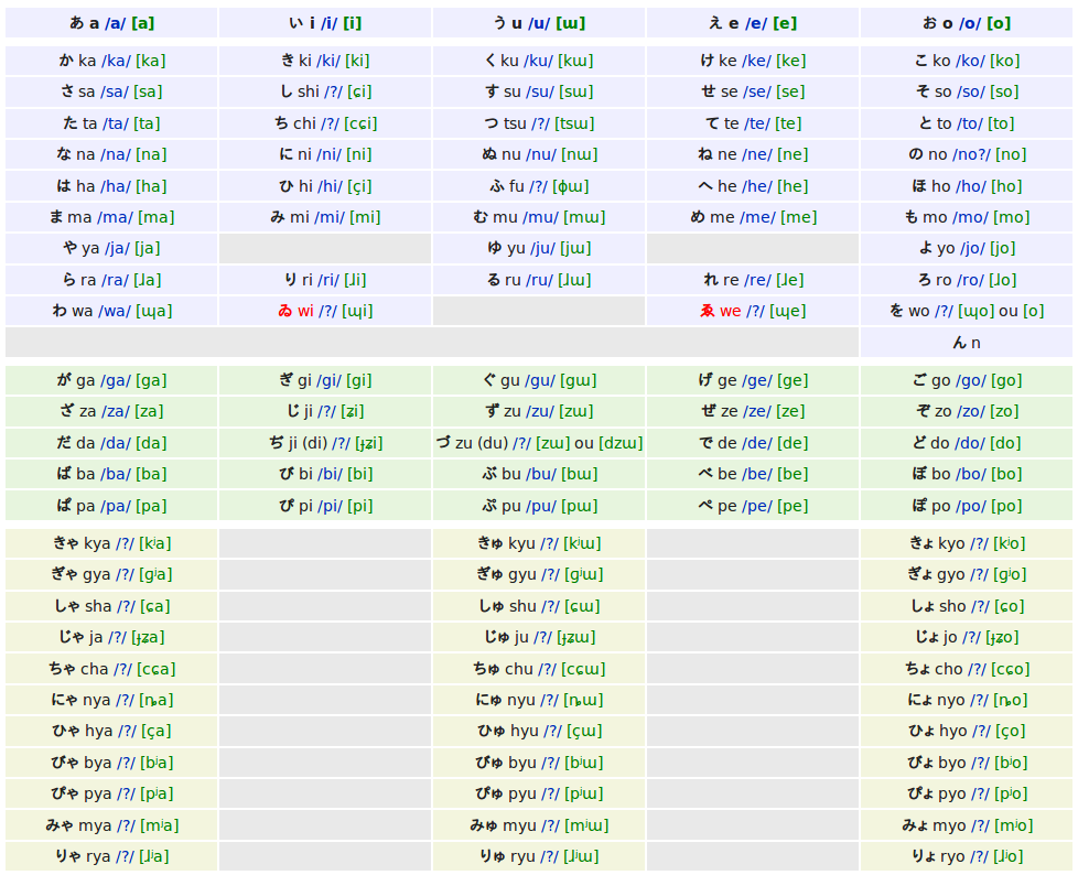
Below is a table showing the hiragana characters and their pronunciation (source).
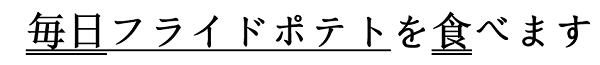
mainichi furaidopoteto o tabemasu / I eat fried potatoes every day
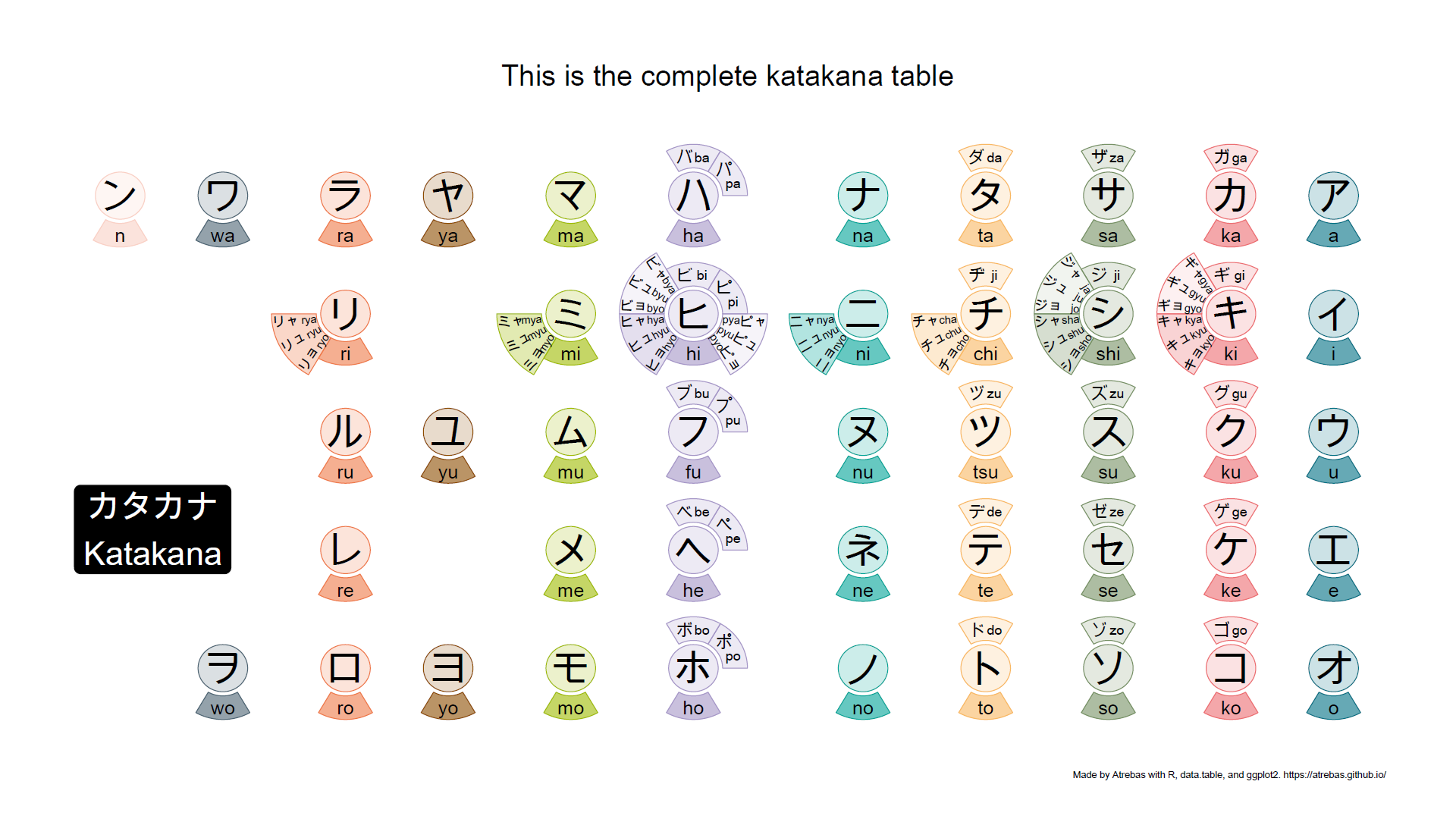
New kana tables
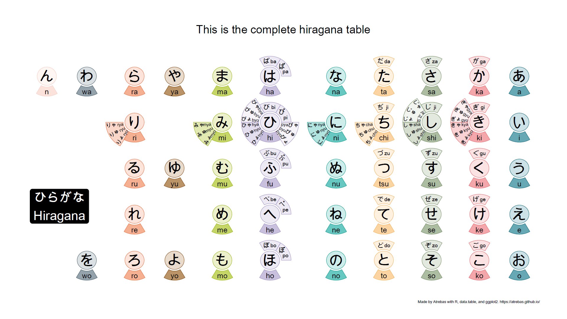
Most of the kana tables, such as the one above, do not properly reflect the rules that apply to these characters. So I tried to build plots to better illustrate the underlying logic. The final result is shown below and available as a pdf file.
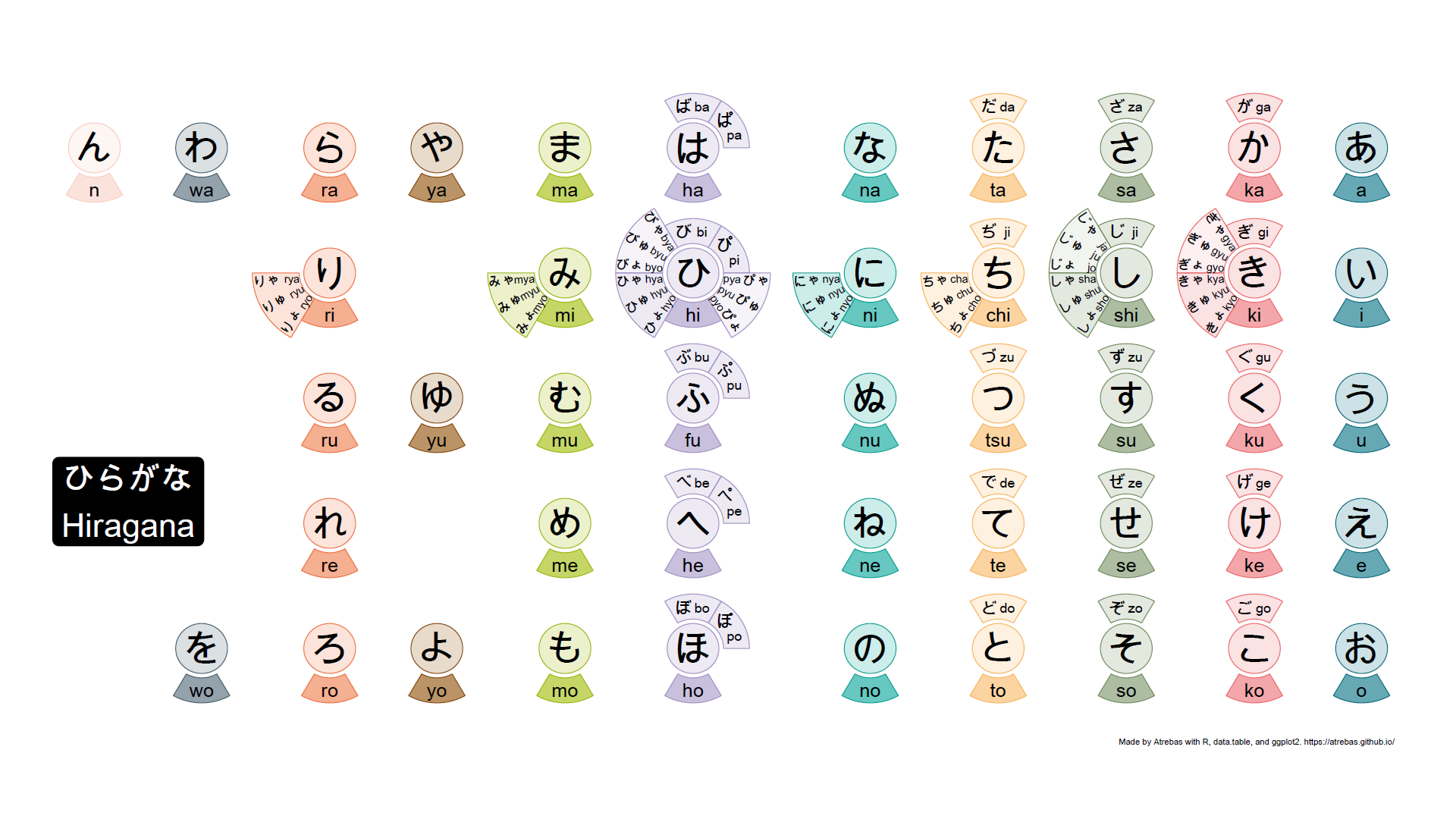
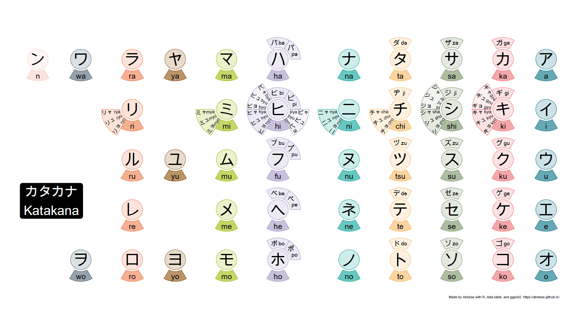
Browse the following image gallery to get further explanations (pdf).
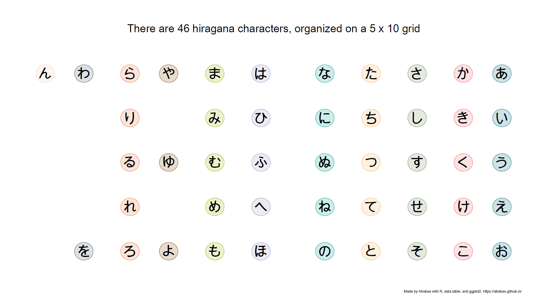
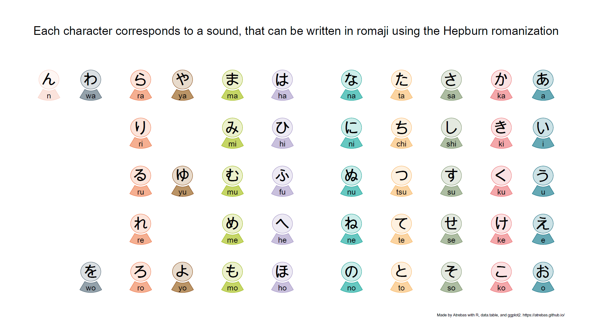
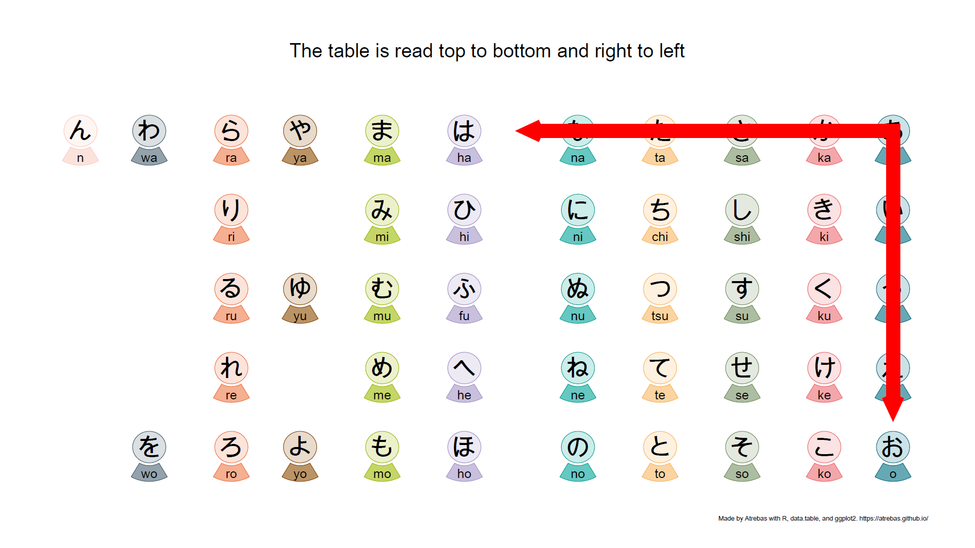
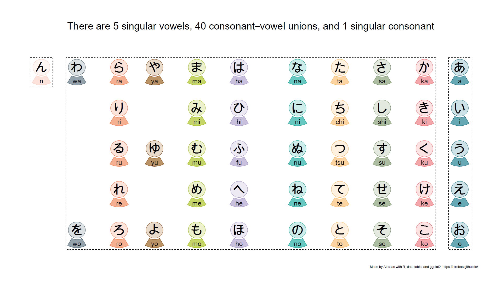
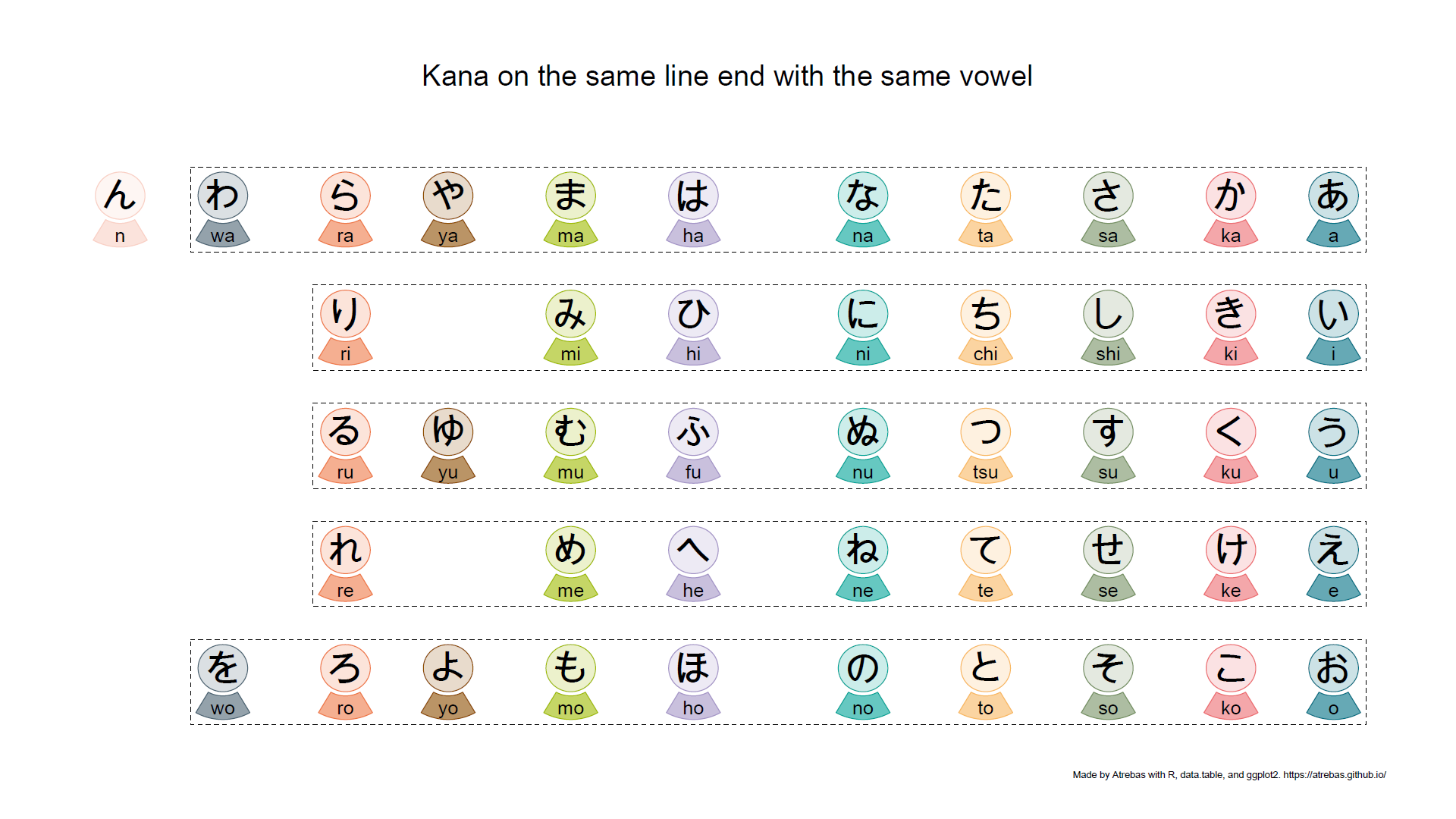
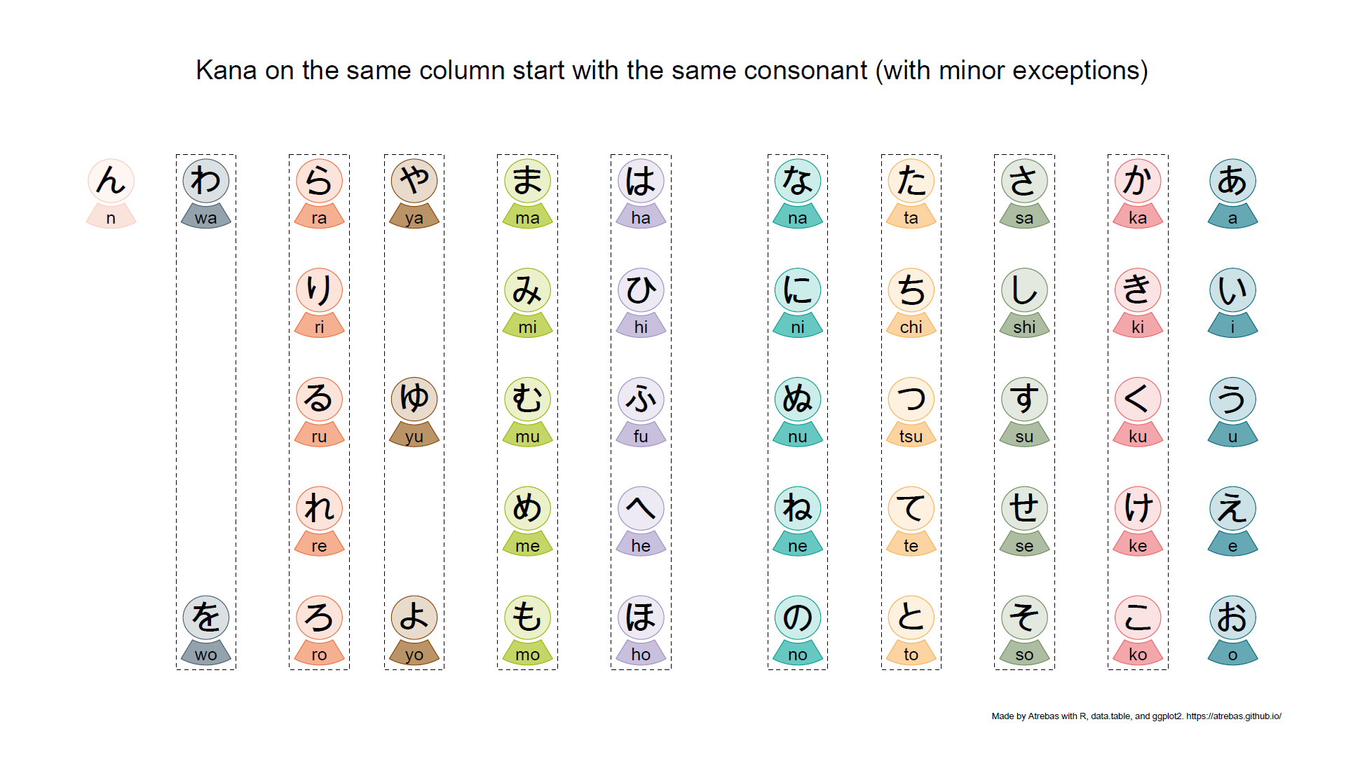

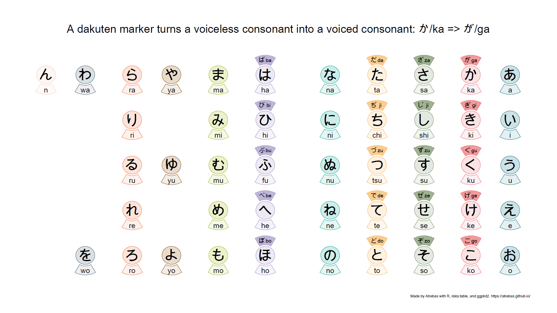
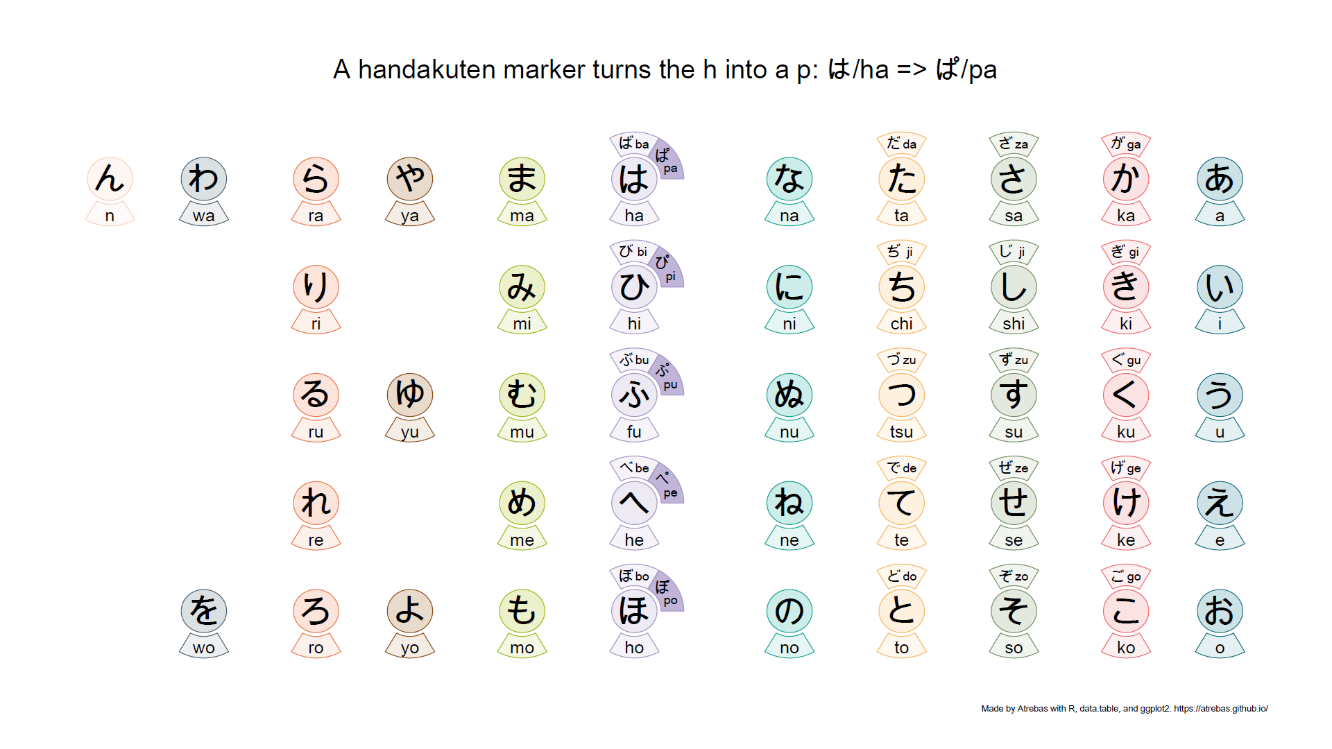
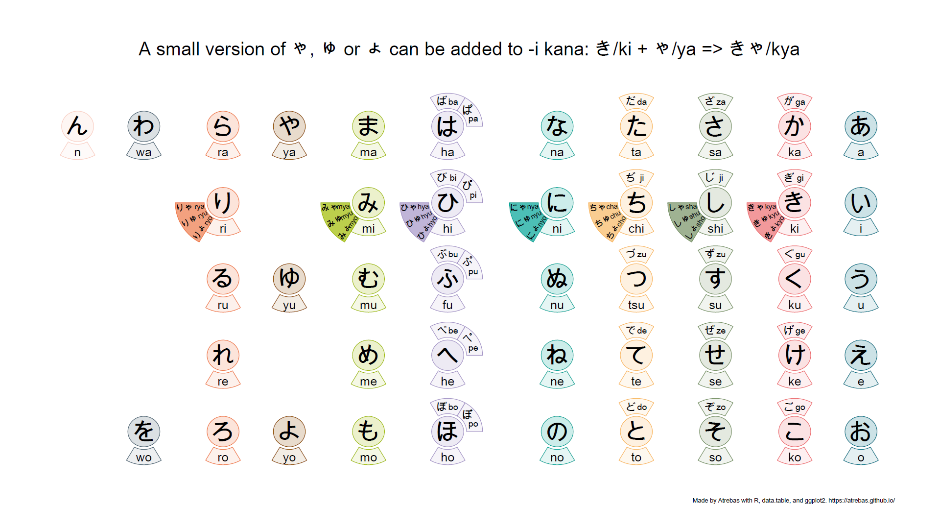
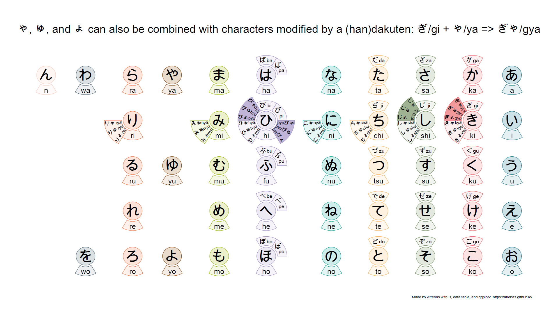
1
There are a few more things to know, related to long vowels, gemination (consonant lengthening), or additional katakana combinations used in modern Japanese. But they are easy to understand once you get the essential rules presented above.
The code
- Initially, I used rbokeh. It is an awesome package, but I finally
switched back to ggplot2 to render the plots as pdf files.
- I explored several possibilities for the polygons, but arcs were more appropriate to fit the text properly.
- I also gave a try to ggpomological, but had some problems to fine-tune the appearance of the plot, so I sticked to a simple style.
- “Data processing” was made smooth with data.table.
- Character encoding is a pain.
- The code that follows has been used to produce the final pdf plots for both hiragana and katakana. The input file with all the characters can be found here.
library(data.table)
library(ggplot2)

kana   <- fread("https://raw.githubusercontent.com/Atrebas/atrebas.github.io/master/files/kana3.csv",
                encoding = "UTF-8")
kana

plot_kana <- function(kana){

  # add columns to make computation and plotting easier
  t1s    <- setNames(c(4, 1, 0, 3, 2, 5) * pi / 3, unique(kana[, grp]))
  alphas <- setNames(c(4, 3, 3, 2, 1, 1),  unique(kana[, grp]))

  kana[, ':='(x     = as.double(x),      # floats will be used to adjust x
              y     = y * 1.15,          # increase y positions
              idx   = 1:.N,              # index for each character
              t1    = t1s[grp],          # arcs start angle
              t2    = t1s[grp] + pi / 3, # arcs end angle
              alpha = alphas[grp],       # arcs group for transparency
              r1    = 0.27,              # arcs inner radius
              r2    = 0.5)]              # arcs outer radius

  # modify youon* text alignment properties
  kana[grepl("youon", grp),
       ':='(r2    = r2 * 1.37,             # increase arcs outer radius
            t3    = (t1 + t2) / 2,         # angle for geom_text
            vjust = rep(c(1, 0.5, 0), 11), # geom_text parameter
            hjust = rep(0:1, c(30, 3)))]   # geom_text parameter

  kana[grepl("youon", grp) & vjust == 1, t3 := c(t1 + 0.05)]
  kana[grepl("youon", grp) & vjust == 0, t3 := c(t2 - 0.05)]
  kana[romaji %in% c("pya", "pyo"), t3 := c(t2[1] - 0.05, t1[2] + 0.05)] # switch


  # circles - one for each kana
  circles <- kana[grp == "none",
                  by = idx,
                  .(xs = x + (r1 * 0.85) * cos(seq(0, 2 * pi, length.out = 100)),
                    ys = y + (r1 * 0.85) * sin(seq(0, 2 * pi, length.out = 100)),
                    x  = x)]

  # arcs - one for each romaji and group (dakuten, youon, ...)
  arcs <- unique(kana, by = c("x", "y", "grp"))
  arcs <- arcs[, by = idx,
               .(xs = x + c(r1 * cos(seq(t1, t2, length.out = 100)),
                            rev(r2 * cos(seq(t1, t2, length.out = 100)))),
                 ys = y + c(r1 * sin(seq(t1, t2, length.out = 100)),
                            rev(r2 * sin(seq(t1, t2, length.out = 100)))),
                 alpha = alpha,
                 x = x)]

  # compute spacing and required ajustment to make it more homogeneous
  ix   <- c(1, 2, 4, 11) # kana with no yuoun will recieve extra space
  adjx <- arcs[, .(xmin = min(xs), xmax = max(xs)), keyby = x]
  adjx[,   adj := 0.2 - c(xmin - shift(xmax))]
  adjx[ix, adj := c(0, na.omit(adj) + 0.25)]
  adjx[,   adj := cumsum(adj)]

  # apply the adjustment (update while joining)
  kana[adjx,     x := x  + i.adj, on = "x"]
  arcs[adjx,    xs := xs + i.adj, on = "x"]
  circles[adjx, xs := xs + i.adj, on = "x"]


  # ----------------------------

  p <- ggplot() +
    # inner circles
    geom_polygon(data = circles,
                 aes(x      = xs,
                     y      = ys,
                     colour = as.factor(x),
                     fill   = as.factor(x),
                     group  = idx),
                 alpha = 0.2) +

    # arcs
    geom_polygon(data = arcs,
                 aes(x      = xs,
                     y      = ys,
                     colour = as.factor(x),
                     fill   = as.factor(x),
                     group  = idx,
                     alpha  = as.factor(alpha))) +

    # text for main kana
    geom_text(data = kana[grp == "none"],
              aes(x        = x,
                  y        = y,
                  label    = kana,
                  fontface = "bold"),
              size = 14.5) +

    # text for main romaji
    geom_text(data = kana[grp == "none"],
              aes(x     = x,
                  y     = y - (r2 + r1) / 2,
                  label = romaji),
              fontface = "bold",
              size     = 7) +

    # text for dakuten
    geom_text(data = kana[grp %in% c("dakuten", "handakuten")],
              aes(x     = x + (r1 + r2) / 2 * cos(t1 + (t2 - t1) * 0.7),
                  y     = y + (r1 + r2) / 2 * sin(t1 + (t2 - t1) * 0.7),
                  label = kana),
              fontface = "bold",
              size     = 6.5) +

    geom_text(data = kana[grp %in% c("dakuten", "handakuten")],
              aes(x     = x + (r1 + r2) / 2 * cos(t1 + (t2 - t1) * 0.3),
                  y     = y + (r1 + r2) / 2 * sin(t1 + (t2 - t1) * 0.3),
                  label = romaji),
              size     = 5,
              fontface = "bold") +

    # text for youon
    geom_text(data = kana[grepl("youon", grp)],
              aes(x     = x + r2 * cos(t3),
                  y     = y + r2 * sin(t3),
                  label = kana,
                  angle = ifelse(t3 < (3 * pi / 2), t3 + pi, t3) * 180 / pi,
                  hjust = hjust,
                  vjust = vjust),
              size     = 5,
              fontface = "bold") +

    geom_text(data = kana[grepl("youon", grp)],
              aes(x     = x + r1 * cos(t3),
                  y     = y + r1 * sin(t3),
                  label = romaji,
                  angle = ifelse(t3 < (3 * pi / 2), t3 + pi, t3) * 180 / pi,
                  vjust = vjust,
                  hjust = 1 - hjust),
              size = 4)

  # theme and title
  title  <- ifelse(kana[1, system] == "hiragana",
                   "ひらがな\nHiragana",
                   "カタカナ\nKatakana")

  colors <- c("#F9D0C5", "#4C6473", "#EE7948", "#8C4C00", "#9FBB00", "#a596c7",
              "#00A497", "#F8B862", "#769164", "#ec6d71", "#007083")

  p <- p +
    theme_void() +
    scale_fill_manual(  values = colors, guide = FALSE) +
    scale_colour_manual(values = colors, guide = FALSE) +
    scale_alpha_manual(values = c(0.1, 0.2, 0.2, 0.6), guide = FALSE) +
    labs(caption = paste("Made by Atrebas with R, data.table, and ggplot2.",
                         "https://atrebas.github.io/",
                         "                         \n")) +
    annotate("label",
             x      = 1.3,
             y      = 2.5,
             label  = title,
             size   = 12,
             fill   = "black",
             colour = "white",
             label.padding = unit(0.7, "lines"),
             label.r       = unit(0.5, "lines"))
  p
}


cairo_pdf(filename = "kana.pdf",
          family   = "Arial Unicode MS",
          width    = 21,
          height   = 10,
          onefile  = TRUE)

print(plot_kana(kana[system == "hiragana"]))
print(plot_kana(kana[system == "katakana"]))

dev.off()